Building on a background in Houdini, simulation, and procedural workflows, I am exploring their close connection to OpenUSD, Physical AI, and digital twins. I am currently learning OpenUSD composition and layering while developing a bridge between procedural Houdini environments and digital-twin simulations in NVIDIA Isaac Sim.
This is one complete run, shown at 2× speed. The PhysX vehicle follows the route exported from Houdini, stops for the NavMesh-driven pedestrian, continues through both turns, and brakes again at the route endpoint. LiDAR drives the stop-and-release logic; the camera is only used to inspect the run. I left the navigation and sensor overlays visible so the test setup can be seen.
From Houdini to a driving test.
I built the street district as a Houdini Digital Asset, with controls for the road layout, buildings, and street furniture. It exports to OpenUSD and becomes the environment for a physical vehicle in Isaac Sim.
The current test combines a predefined route, a PhysX vehicle, RTX LiDAR, and a pedestrian walking on a baked NavMesh. When the pedestrian enters the car’s forward detection area, the controller applies the brake and waits for new LiDAR returns before moving again.
These are the controller settings used in the recorded run, not performance guarantees. The braking threshold also increases with vehicle speed. The crossing sequence worked in this test; I have not yet run a larger repeatability study.
SENSING AND RESPONSE
How the car handles the crossing
For this test, the pedestrian crosses on a baked navigation surface while the vehicle approaches in its lane. The controller checks fresh LiDAR returns inside a narrow area ahead of the car and overrides the driving commands when that area is occupied.
01 / APPROACH
Follow the route
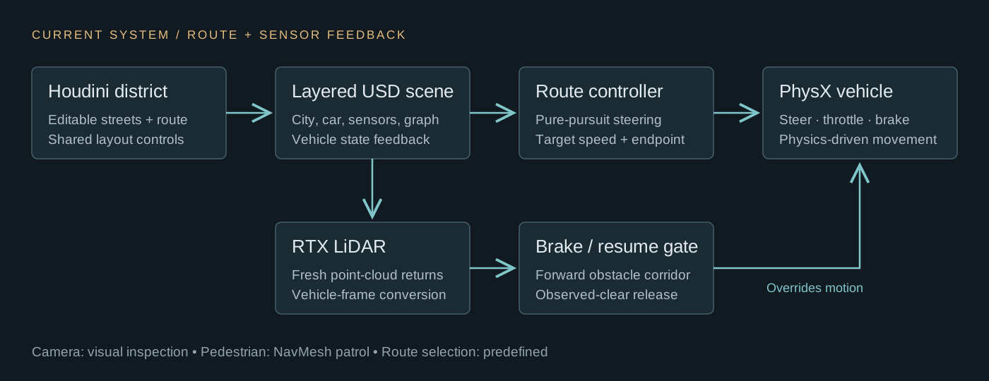
Vehicle position, orientation, and velocity feed a pure-pursuit controller. Steering, accelerator, and brake commands flow through an Action Graph into the PhysX vehicle.
02 / YIELD
Brake for occupied space
Fresh LiDAR points are transformed into the vehicle frame. A forward corridor rejects road and chassis returns, then measures obstacle clearance. The crossing test produced a full brake command and a visible stop.
03 / CONTINUE
Wait for clear evidence
The controller holds the stop while space remains blocked or uncertain. New returns beyond the previously blocked location must confirm clearance before driving resumes. The car continued after the pedestrian cleared the lane.
Controller architecture diagram. The camera currently provides a visual view; LiDAR supplies the obstacle measurements used by the braking logic.
BUILT IN HOUDINI
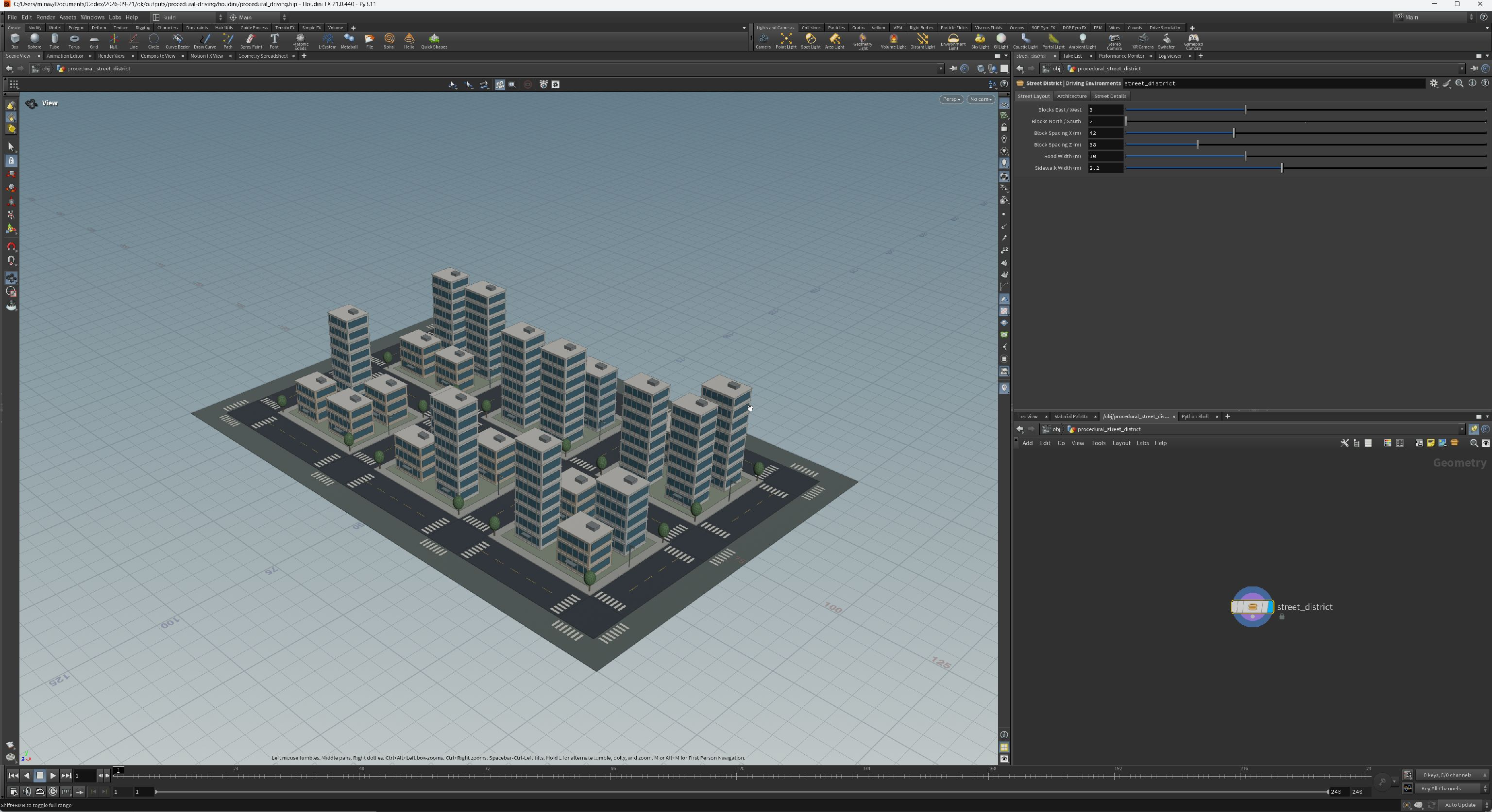
A district controlled by an HDA
01
Lay out the streets
The procedural layout generates the street network, raised sidewalks, block parcels, markings, and crossings. Block count, spacing, road width, and sidewalk width remain editable.
02
Vary the architecture
Three building modules combine floor bands, glazing, roof equipment, and entry canopies. Seeded variant selection and Attribute Randomize change their distribution and footprints across the generated building sites.
03
Export the cooked result
The native USD File Export node writes named geometry groups and display colors. Metres and Y-up are preserved in Isaac Sim, where static collision surfaces and vehicle physics are added.
HDA controls and the cooked district in Houdini. Select the image to inspect the interface at full resolution.
OPENUSD HANDOFF
From HDA to simulation
The HDA writes the city geometry and route points to a dedicated environment USD file. I keep the car, collision overrides, sensors, and Action Graph in a separate simulation layer. This lets me re-export the Houdini environment without rebuilding the vehicle setup. When the route changes, a reset branch reads its new starting point and direction, places the car above the road, and clears its velocity. I tested the link by changing the block spacing in Houdini and reloading the export in Isaac Sim.
ISAAC SIM / ACTION GRAPH
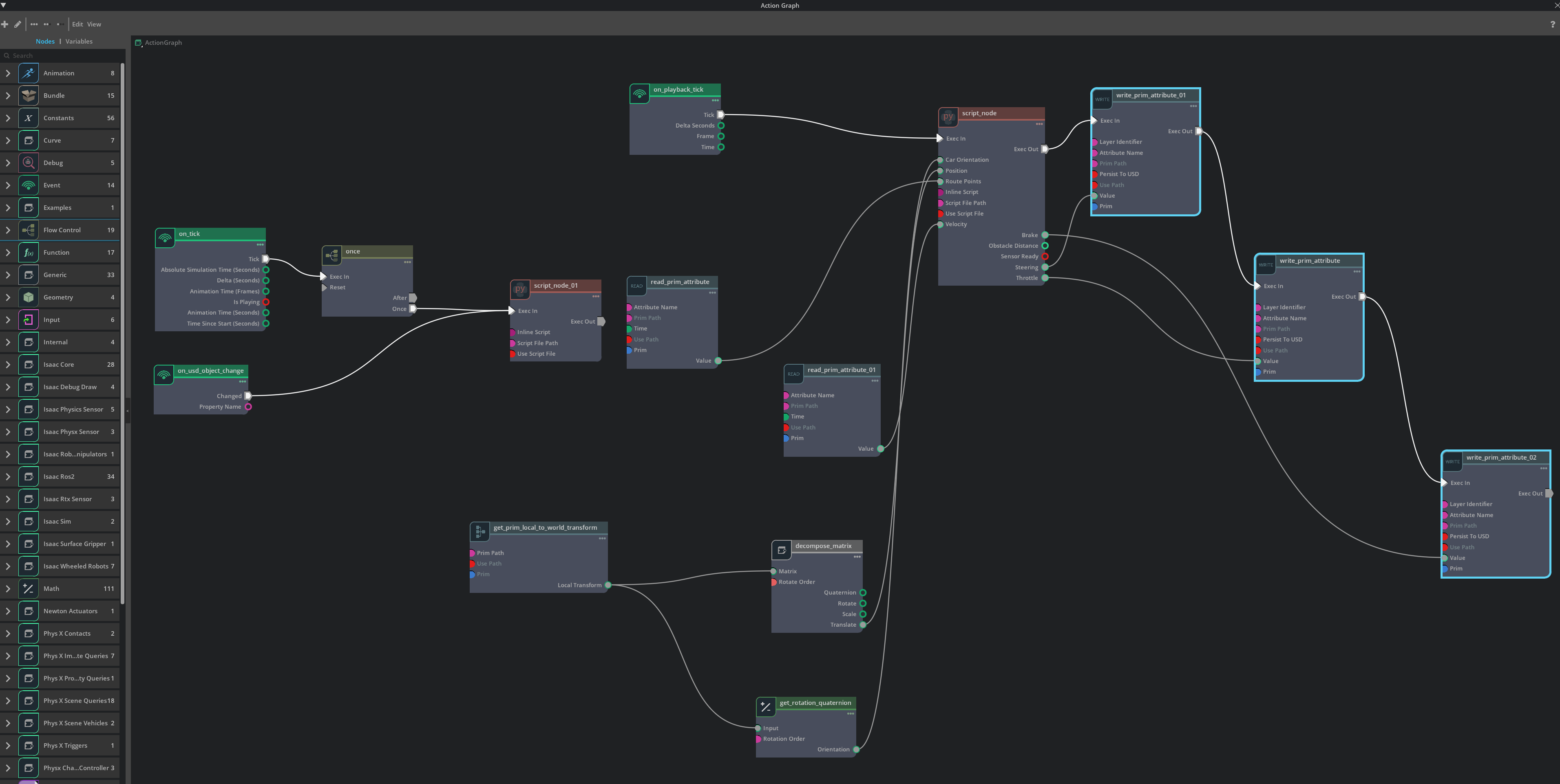
The driving and reset graph
The actual project graph. Route points, position, orientation, and velocity feed the driving Script Node. Its outputs command steering, throttle, and brake through three sequential Write Prim Attribute nodes. The left branch handles initial placement and route-change resets. The controller also exposes obstacle distance and sensor readiness. Select the image to inspect the full-resolution graph.
DEVELOPMENT PROCESS
What I built and tested
01 / SCENE COMPOSITION
Keep the city editable
Separate environment exports from simulation authoring. Link the road layout and route to shared Houdini controls, reload the environment layer, and reset the vehicle from the updated route instead of entering coordinates manually.
02 / PHYSICS AND FEEDBACK
Build a physical driving loop
Add static collisions to roads, sidewalks, buildings, and street furniture. Configure the vehicle chassis, wheels, suspension, and steering, then connect route and vehicle state to the driving controller.
03 / SENSOR INTEGRATION
Check what the LiDAR sees
Parent the camera and LiDAR to the vehicle and position their mounts. Inspect the point cloud, resolve sensor and vehicle coordinate frames, and filter chassis and ground returns. Stationary scans expose missed obstacles and close-range visibility limits before another driving test.
04 / PEDESTRIAN NAVIGATION
Connect both sides of the crossing
Bake a walkable NavMesh for an Actor SDG patrol. Compare a simple test surface with the exported meshes, correct winding on navigation test copies, and exclude painted markings that fragmented the walking surface. A path query then connects both sides on the same navigation island.
05 / BRAKING AND RESUME
Separate absence from clearance
Use a minimum four-metre trigger with a speed-dependent stopping margin. Hold braking through uncertain scans and require fresh evidence beyond the blocked location before release. Test the sequence with a stationary cube, then a walking pedestrian.
06 / REPEATABLE SETTINGS
Verify the active behavior
Check the pedestrian’s authored patrol speed rather than relying only on the setup panel. Existing actors retain their scene behavior when setup skips respawning them. Save the corrected behavior and reload the scene before testing the next crossing.
Current result
In the recorded crossing run, the brake output reached 1 and the car stopped before the pedestrian. It moved again after the lane cleared. The system only detects occupied space; it does not identify pedestrians, choose its own route, or represent a complete autonomous-driving stack.
TECHNICAL NOTES
Environment tools meet vehicle control
What is procedural?
The city layout HDA is generated procedurally in Houdini. Python assembles the node graph; native Houdini operators cook the geometry. Six validation cases check repeatable seeds, alternate seeds, expanded layouts, tight block dimensions, and disabled street details.
How does the car drive?
A pure-pursuit controller turns route error into steering, and a speed controller supplies throttle and braking. The current implementation uses RTX LiDAR measurements to gate these commands when the forward corridor is blocked. Native graph nodes read the vehicle state and apply the outputs of a Python Script Node. Physics determines the motion through the wheels, suspension, and tire forces. The car uses simulator pose and an exported route; independent route selection is still planned.
Scope, attribution, and next steps
The Houdini district, HDA, vehicle appearance, route controller, test setup, and analysis form this personal study. The physical vehicle is configured with NVIDIA’s PhysX vehicle tooling. The environment is fictional, with no calibrated real-world twin. The camera, RTX LiDAR, and navigation-driven pedestrian form the sensing and interaction setup. The pedestrian uses a supplied NVIDIA character asset. The camera is available for inspection but does not yet classify road users. Next steps are repeatable crossing scenarios, destination and route planning, traffic rules, and perception from sensor observations. The current corridor filter is designed for a small, flat-road experiment and is not a complete collision predictor for turns.
STUDY 02 / ISAAC SIM
Procedural Robotics Test Cell
Simulation study
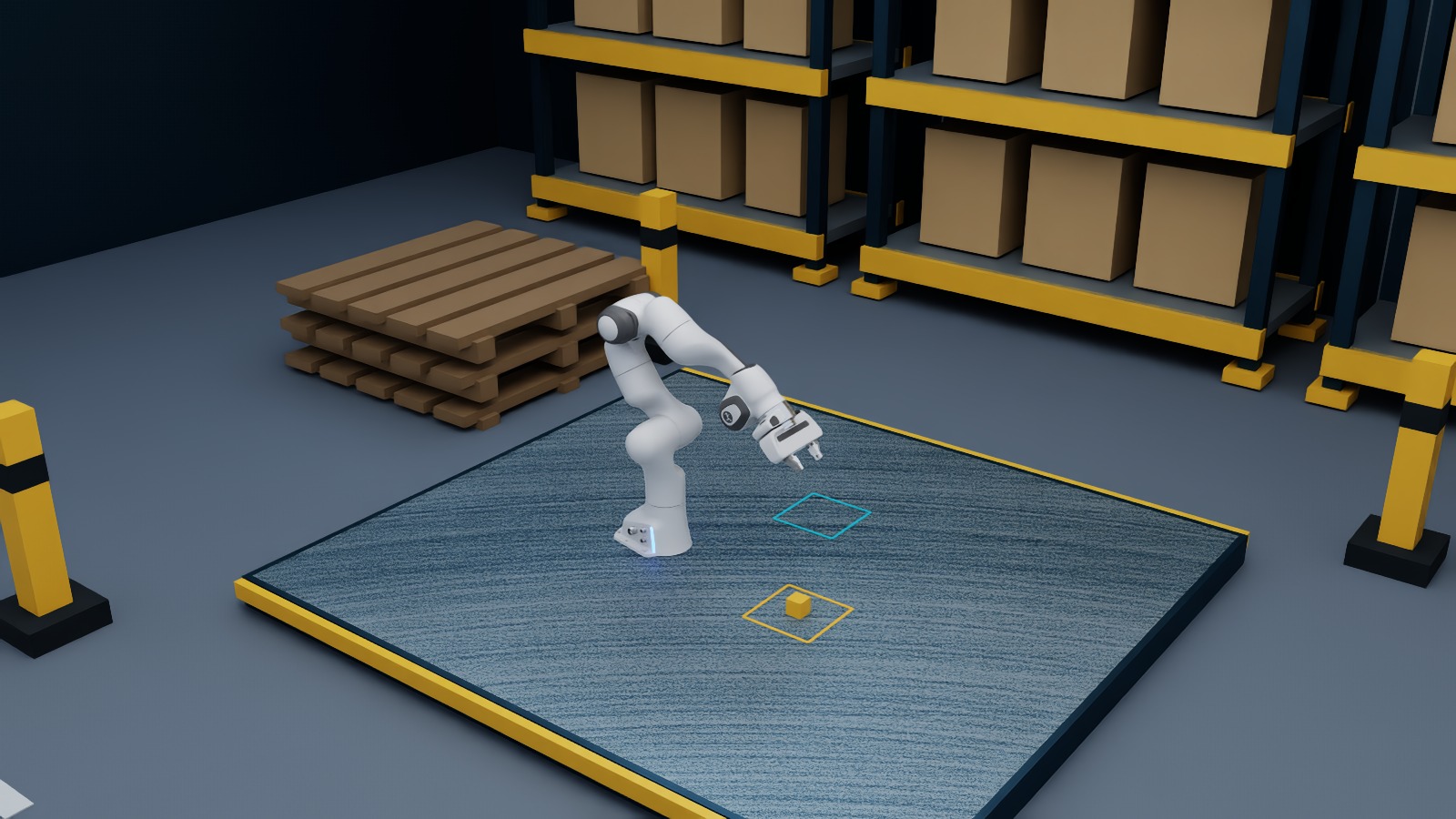
01 — The work cellActual Isaac Sim render
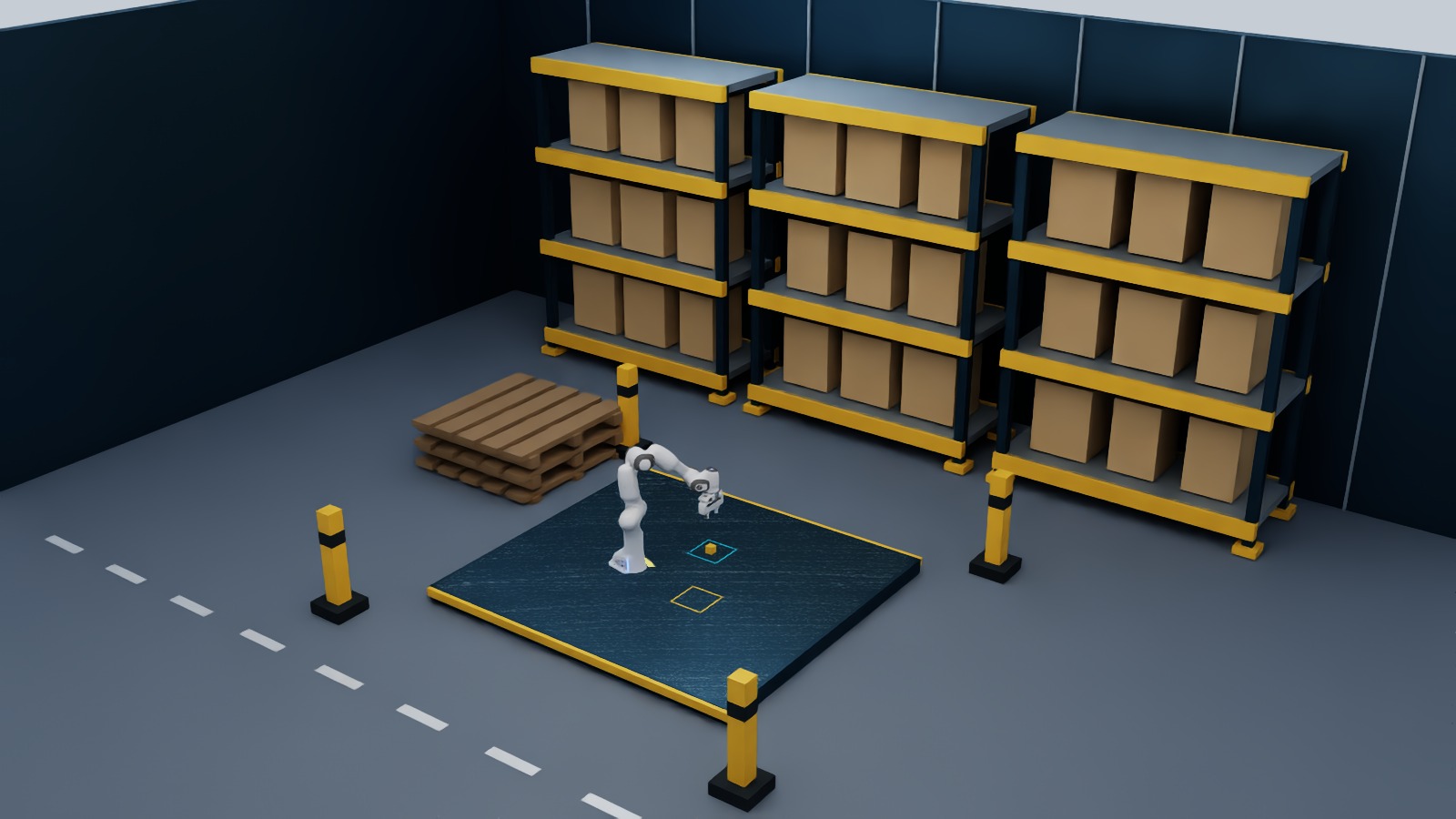
A reusable Isaac Sim test cell.
I built this small warehouse scene to practice assembling an OpenUSD environment, controlling a robot, and measuring the result in one repeatable setup.
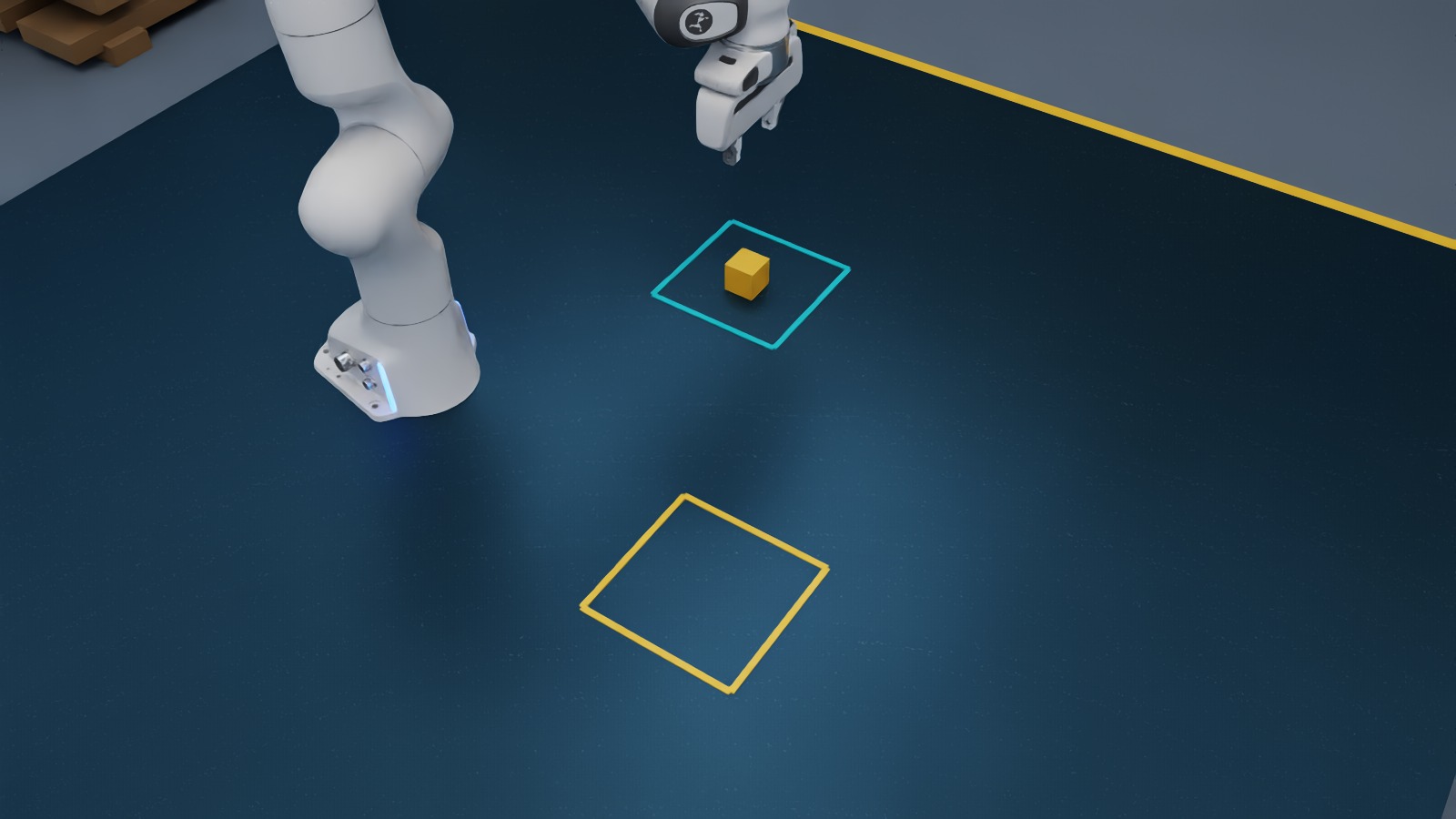
A Franka Panda moves a physical workpiece between marked zones. Each run records the object trajectory, robot joint positions, lift height, and placement error.
OpenUSDIsaac Sim 6.0.1PythonPhysXDifferential IK
12evaluated trials
12 / 12successful placements
11.3 mmmean placement error
3scenario variants
12 deterministic simulation trials across three pickup scenarios. Success: lift above 12 cm, final XY error below 6 cm, final height within 4 cm. These runs are a small experiment, not a production reliability estimate.
SEE IT RUN
From approach to release
Recorded in Isaac Sim. The object moves through physical contact with the gripper. The controller uses smooth waypoints and differential inverse kinematics.
THE WORKFLOW
Build. Simulate. Measure.
01
Procedural scene
Python generates the facility, safety markings, pallet stack, and storage modules. OpenUSD references and instancing keep the rack asset reusable.
02
Physical behavior
An articulated arm, collision shapes, gravity, and a dynamic workpiece form the test. A waypoint state machine drives the robot through a complete transfer.
03
Recorded evidence
Seeded scenarios vary the pickup location and lighting. Telemetry captures the actual motion, and an explicit geometric check determines success.
A personal study covering procedural scene construction, scenario setup, experiment harness, telemetry, and presentation. The robot asset and differential IK helper come from NVIDIA’s installed Isaac Sim examples. The environment is authored with Python/OpenUSD; a Houdini export is a future extension.
What counts as success?
The object must lift above 12 cm, finish within 6 cm of the target in the horizontal plane, and settle within 4 cm of the target height. Finishing the controller sequence alone does not count. The downloadable results include each trial’s final position and lift height.
Limits & next experiment
This is a fictional cell for studying digital-twin workflows. It has no calibrated physical counterpart and makes no sim-to-real claim. Control uses known object poses, rather than visual perception. No reinforcement-learning policy was trained in Isaac Lab. Study 03 below extends this foundation with camera-based sorting and visual verification.
Implementation notes
Scene generation, the saved USD stage, and the experiment harness are maintained together. The study was run in Isaac Sim 6.0.1 with the Franka asset from NVIDIA’s asset library. Per-trial results and telemetry are available below.
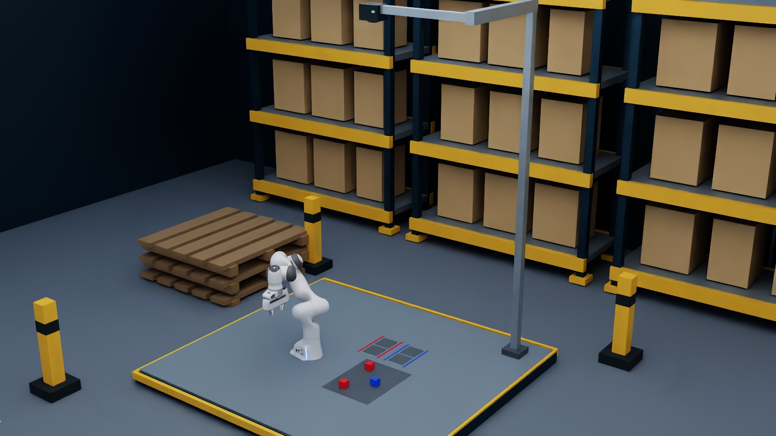
01 — From pixels to physical actionActual Isaac Sim render
Sorting from camera observations.
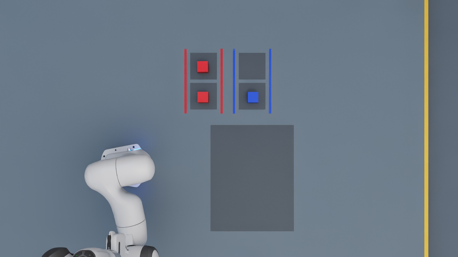
I extended the test cell with an overhead camera so the robot could locate its pickup targets from RGB images instead of using the known scene position directly. Three colored parts are sent to two receiving lanes.
After each transfer, the arm moves out of the camera view and the controller checks the destination before continuing.
3 of 3 episodes completed all three placements. Each transfer requires the correct class, a physical lift, a placement within the geometric tolerances, and camera confirmation. This is a small controlled experiment.
SEE IT RUN
Three parts. Two destinations.
Actual PhysX manipulation recorded in Isaac Sim. Three manipulation excerpts are joined together; approach, retraction, settling, sensor-acquisition pauses, and arm-parking motions are omitted. Parts remain dynamic throughout each grasp.
THE CONTROL LOOP
A decision at every step
01 / OBSERVE
Pixels to positions
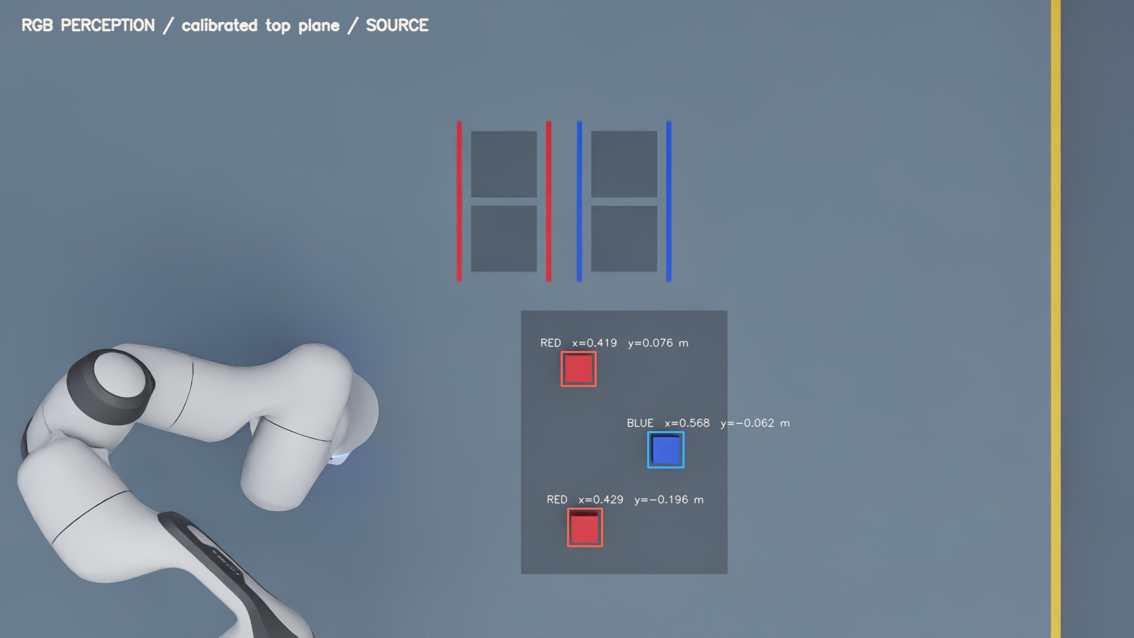
HSV color segmentation finds candidate parts in the input region. A calibrated pinhole projection maps image centroids onto the known part-height plane.
02 / ACT
Class to destination
A queue assigns each detection to an available slot in its color lane. Smooth Cartesian waypoints and differential IK drive the physical grasp and transfer.
03 / VERIFY
Check before continuing
A second RGB observation looks for the matching color at the destination. Missing detections or an unconfirmed placement stop the episode.
02 — What the detector seesRGB image + computed annotations03 — The final arrangementCamera view after evaluation
TECHNICAL NOTES
A more complete experiment
What changed from study 02?
The procedural warehouse becomes a vision-guided work cell with a camera gantry, input tray, two receiving lanes, and three dynamic parts. The new work adds RGB detection, image-to-world projection, destination-slot allocation, visual feedback, and separate localization and manipulation metrics.
How are the results measured?
Three seeded conditions vary pickup layout and lighting. The controller uses image-derived pickup coordinates. Simulator object positions are read separately for reset and scoring. Success requires a lift above 12 cm, final XY error below 6 cm, final height within 4 cm, correct color classification, and visual confirmation within 6.5 cm.
Assumptions & limits
The detector assumes known part height, two distinctive colors, a fixed calibrated camera, and an unobstructed input region. It uses classical image processing. This study does not include a trained vision model, collision-aware path planner, real-robot validation, or Isaac Lab policy training.
Implementation notes
The scene generator, camera parameters, and controller share the warehouse foundation from study 02. Tested in Isaac Sim 6.0.1 using NVIDIA’s referenced Franka asset and differential IK helper. Per-transfer results and telemetry are available below.
I trained a Unitree G1 balance controller from scratch, beginning with small disturbances and increasing their strength as training progressed.
The PPO policy adjusts twelve leg joints from body motion and joint feedback. I compared it with fixed posture, the original untrained network, and frozen trained targets under the same disturbance schedule.
Isaac LabUnitree G1PPO / RSL-RLPyTorchPhysX
19.7Mtraining transitions
46 / 64trained-policy test survivals
1,024parallel training environments
12learned leg-joint actions
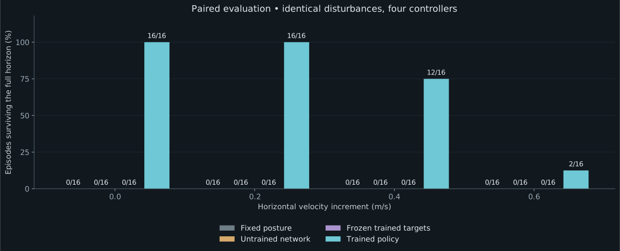
64 held-out simulation episodes per controller, with four disturbance levels. Survival means reaching 9.98 seconds without a fall or excessive drift. One training seed; this is a controlled experiment, not a hardware reliability claim.
WATCH THE COMPARISON
Same disturbance. Different response.
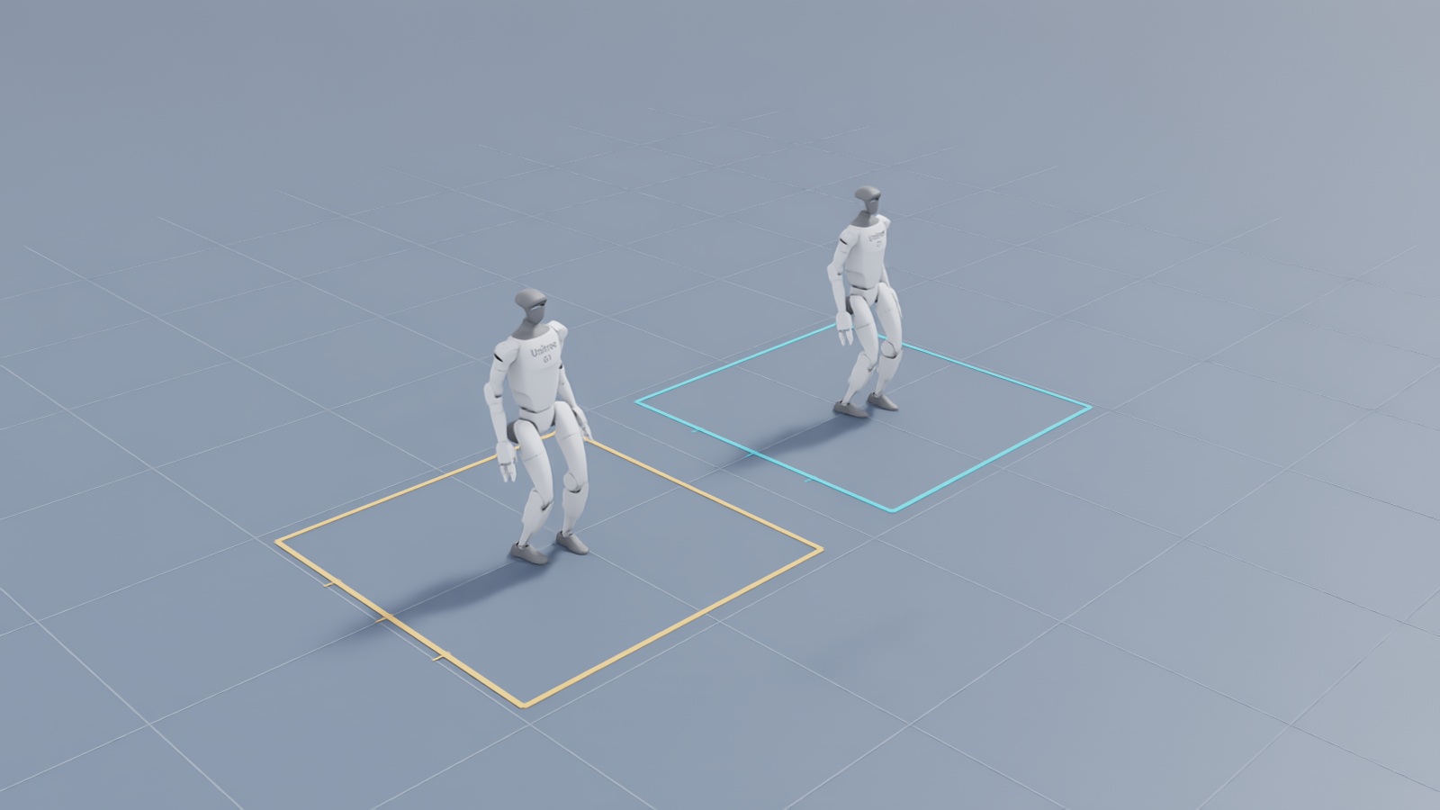
Amber: trained targets frozen at 1.5 seconds.Cyan: trained policy. Continuous physics simulation, captured at 25 fps. Both begin with trained feedback; the amber controller then holds its last targets. This illustrative rollout uses level initial poses and is separate from the randomized evaluation. Both receive a 0.4 m/s horizontal velocity increment at 2 seconds and the opposite increment at 5 seconds. These are controlled simulation disturbances, not calibrated physical pushes.
THE LEARNING PROCESS
From falling to balancing
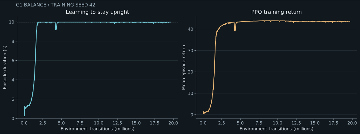
Logged PPO training feedback. Episode duration is capped at 9.98 seconds; the curves show a rolling average of completed episodes. Disturbance strength increases during training.
01
Define the task
Body velocity, projected gravity, leg-joint state, and previous actions form 45 observations. The policy produces bounded joint offsets; the upper body holds its nominal pose.
02
Train with a curriculum
PPO learns across 1,024 parallel environments. Random starting tilt and disturbances encourage feedback control. The maximum disturbance rises from 0.10 to 0.45 m/s.
03
Test against baselines
All four controllers face the same held-out directions and timings. The frozen-target baseline isolates the benefit of continued feedback after 1.5 seconds. Tests include 0.60 m/s disturbances, beyond the maximum used during training.
MEASURED RESULTS
Does learning improve survival?
Sixteen episodes per disturbance level for each controller. Fixed posture: 0 / 64 overall. Untrained network: 0 / 64. Frozen trained targets: 0 / 64. Trained policy: 46 / 64. Results stop at the first failure. Baselines may fall before the first disturbance. The trained policy passed 16/16 at both lower levels, 12/16 at 0.4 m/s, and 2/16 at 0.6 m/s.
TECHNICAL NOTES
A reproducible learning experiment
What is trained?
A 45-input, 12-output neural network, initialized from scratch and optimized with PPO. Its hidden layers have 128, 128, and 64 units. It controls leg-joint targets at 50 Hz; PhysX runs at 200 Hz. The inference export includes the learned observation normalization.
What counts as a successful test?
The humanoid must remain above 0.48 m pelvis height, below roughly 49.5° of tilt, and within 1.5 m of its starting position for 9.98 seconds. Disturbances occur at 2 and 5 seconds. The second is opposite to the first. Starting tilt and horizontal velocity vary under a separate test seed. Survival does not require returning to the exact starting pose.
What does this project add?
The balance task, reward design, disturbance curriculum, paired evaluation, data analysis, and presentation. The G1 model and joint-drive configuration come from NVIDIA Isaac Lab; PPO comes from ETH Zurich and NVIDIA’s RSL-RL.
What are the limits?
This is simulated standing balance with one training seed and ideal state feedback. It does not demonstrate walking, getting up after a fall, navigation, or real-robot deployment. Broader tests would vary mass, friction, sensor noise, and control latency, then repeat training with additional seeds.